In this article, the method is considered as a way to solve systems. linear equations (Slava). The method is analytic, that is, it allows you to write a solution algorithm in general, and then substitute the values \u200b\u200bthere from specific examples. In contrast to the matrix method or formulas, when solving a system of linear equations, the Gauss method can also be operated with those that have solutions infinitely a lot. Or do not have it at all.

What does it mean to solve the Gauss method?

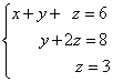
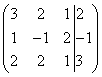
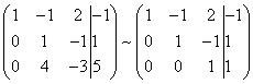
First, you need to write our system of equations to look like this. The system is taken:

The coefficients are recorded in the form of a table, and on the right of a separate column - free members. A column with free members is separated for the convenience of a matrix, which includes this column, is called extended.

Next, the main matrix with coefficients should be brought to the upper triangular form. This is the main point of the system solution by Gauss. Simply put, after certain manipulations, the matrix should look so that some zeros stood in its left lower part:

Then, if you write a new matrix again as a system of equations, it can be noted that in the last line it already contains the value of one of the roots, which is then substituted into the equation above, is another root, and so on.

This description of the solution by Gauss method in the most general features. And what happens if suddenly the system has no solution? Or are they infinitely a lot? To respond to these and many more questions, it is necessary to consider separately all the elements used by solving the Gauss method.

Matrixes, their properties

Nic hidden meaning There is no matrix. This is just a convenient way to write data for subsequent operations with them. They do not even need to be afraid of schoolchildren.

The matrix is \u200b\u200balways rectangular, because it is so more convenient. Even in the Gauss method, where everything comes down to the construction of a triangular matrix, a rectangle appears in the record, only with zeros on the place where there are no numbers. Zeros can not be recorded, but they are meant.

The matrix is \u200b\u200bof size. Its "width" is the number of rows (M), "Length" - the number of columns (N). Then the size of the matrix A (for their designation, capital latin letters are commonly used) will be denoted as a M × n. If m \u003d n, then this matrix is \u200b\u200bsquare, and m \u003d n is its order. Accordingly, any element of the matrix A can be denoted through the number of its row and column: a XY; X - Row number, varies, y - the column number, varies.

B is not the main point of the decision. In principle, all operations can be performed directly with the equations themselves, but the recording will turn out much more cumbersome, and it will be much easier to get confused.

Determinant

Still the matrix has a determinant. This is a very important characteristic. It is not worth finding out that it is not worth it, you can simply show how it is calculated, and then tell what properties of the matrix it determines. The easiest way to find the determinant - through the diagonal. Imaginary diagonals are carried out in the matrix; The elements on each of them are multiplied, and then the obtained works are folded: diagonals with a slope to the right - with a "plus" sign, with a slope to the left - with a "minus" sign.

It is extremely important to note that the determinant can only be calculated at the square matrix. For a rectangular matrix, you can do the following: from the number of rows and number of columns to choose the smallest (let it be k), and then in the matrix it is randomly noted by k columns and k rows. Elements that are on the intersection of selected columns and rows will make a new square matrix. If the determinant of such a matrix is \u200b\u200ba number other than zero, it will be called a basic minor of the original rectangular matrix.

Before proceeding with the solution of the system of equations by Gauss, does not prevent the identifier. If it turns out to be zero, you can immediately say that the matrix has the number of solutions or infinitely, or there are no. In such a sad case, you need to go further and recognize about the rank of the matrix.

System classification

There is such a concept as the rank of the matrix. This is the maximum order of its determinant other than zero (if you remember about the basic minor, it can be said that the rank of the matrix is \u200b\u200bthe order of the base minor).

By how things are dealing with the rank, you can divide the slick on:

• Joint. W. The collaborative rank systems of the main matrix (consisting only of coefficients) coincides with the rank of expanded (with a column of free members). Such systems have a solution, but optionally one, so additionally, joint systems are divided into:
• - defined - Having a single solution. In certain systems, the rag of the matrix and the number of unknown (or the number of columns, which is the same);
• - uncertain - With an infinite number of solutions. The rank of matrices in such systems is less than the number of unknown.
• Incomplete. W. These systems ranks of the main and extended matrices do not coincide. Dysflower solutions do not have.

The Gauss method is good because it allows during the solution to obtain either the unequivocal proof of system incompleteness (without calculating the determinants of large matrices), or the solution in general form for a system with an infinite number of solutions.

Elementary transformations

Before proceeding directly to solving the system, it can be made less cumbersome and more convenient for computing. This is achieved by elementary transformations - such that their execution does not change the final answer. It should be noted that some of the above elementary transformations are valid only for matrices, the sources of which served exactly the Slava. Here is a list of these transformations:

1. Rearranged lines. Obviously, if in the recording of the system to change the order of equations, then it will not affect the solution. Consequently, in the matrix of this system you can also change the lines, not forgetting, of course, about the column of free members.
2. Multiplying all row elements on some coefficient. Very helpful! With it, you can reduce large numbers in the matrix or remove zeros. Many solutions, as usual, will not change, and further operations will be more convenient. The main thing is that the coefficient is not equal to zero..
3. Removing rows with proportional coefficients. This is partly follows from the previous point. If two or more rows in the matrix have proportional coefficients, then when multiplying / dividing one of the rows to the proportionate coefficient, two (or, again, more) are completely identical lines, and you can remove extra, leaving only one.
4. Remove zero string. If during the transformations somewhere it turned out a string in which all elements, including a free member, zero, then such a string can be called zero and throw out from the matrix.
5. Adjustment to the elements of one line of the elements of another (according to the corresponding columns) multiplied by some coefficient. The most uncomfortable and most important transformation of all. It should be part more.

Refridgeing a string multiplied by the coefficient

For simplicity of understanding, it is worth disassembling this process in steps. Two lines from the matrix are taken:

a 11 A 12 ... A 1N | B1.

a 21 A 22 ... A 2N | B 2.

Suppose it is necessary to add the first to the second, multiplied by the coefficient "-2".

a "21 \u003d A 21 + -2 × A 11

a "22 \u003d A 22 + -2 × A 12

a "2N \u003d A 2N + -2 × A 1N

Then in the matrix, the second line is replaced with a new one, and the first remains unchanged.

a 11 A 12 ... A 1N | B1.

a "21 A" 22 ... A "2N | B 2

It should be noted that the multiplication coefficient can be chosen in such a way that, as a result of the addition of two lines, one of the elements of the new line was zero. Therefore, it is possible to obtain an equation in the system, where one unknown will be less. And if you get two such equations, then the operation can be done again and get the equation that will contain already two unknown less. And if each time it turns into zero one coefficient in all lines, which is below the original, then you can, like along the steps, go down to the very nose matrix and get an equation with one unknown. This is called solving the system by Gauss.

In general

Let there be a system. It has M equations and N roots-unknown. Record it as follows:

The main matrix is \u200b\u200bcompiled from the system coefficients. A column of free members is added to the extended matrix and for convenience is separated by a feature.

• the first line of the matrix is \u200b\u200bmultiplied by the coefficient k \u003d (-a 21 / a 11);
• the first modified string and the second line of the matrix are folded;
• instead of the second row in the matrix, the result of the addition from the previous paragraph is inserted;
• now the first coefficient in the new second line is a 11 × (-a 21 / a 11) + a 21 \u003d -a 21 + a 21 \u003d 0.

Now the same series of transformations is performed, only the first and third lines are involved. Accordingly, in each step of the algorithm, the element A 21 is replaced by a 31. Then everything is repeated for A 41, ... A M1. As a result, a matrix is \u200b\u200bobtained, where in the lines the first element is zero. Now you need to forget about the number one string and perform the same algorithm starting from the second line:

• coefficient k \u003d (-a 32 / a 22);
• with the "current" string folds the second modified line;
• the result of the addition is substituted into the third, fourth and so on line, and the first and second remain unchanged;
• in the lines of the matrix, the first two elements are zero.

The algorithm must be repeated until the coefficient K \u003d (-a M, M-1 / A mm) appears). This means that the last time the algorithm was performed only for the lower equation. Now the matrix looks like a triangle, or has a stepped shape. In the bottom line there is equality a Mn × x n \u003d b m. The coefficient and free member are known, and the root is expressed through them: x n \u003d b m / a Mn. The resulting root is substituted into the upper string to find X n - 1 \u003d (B M-1 - A M-1, N × (B M / A Mn)) ÷ A M-1, N-1. And so on, by analogy: In each next line, there is a new root, and, having come to the "top" of the system, you can find many solutions. It will be the only one.

When there are no solutions

If, in one of the matrix lines, all elements, in addition to the free member, are zero, the equation corresponding to this line looks like 0 \u003d b. It has no solution. And since such an equation is enclosed in the system, the many solutions of the entire system are empty, that is, it is degenerate.

When solutions are an infinite amount

It may turn out that in the reduced triangular matrix there are no rows with one element-coefficient of the equation, and one-free member. There are only such lines that, when rewriting, would have the type of equation with two or more variables. So, the system has an infinite number of solutions. In this case, the answer can be given as a general solution. How to do it?

All variables in the matrix are divided into basic and free. The basic are those that stand "with the edge" of rows in a stepped matrix. The rest are free. In the general solution, the basic variables are recorded through free.

For convenience, the matrix first corresponds to the system of equations. Then in the last one, where only one basic variable remained, it remains on the one hand, and everything else is transferred to another. This is done for each equation with one basic variable. Then in the remaining equations, where it is possible, instead of the basic variable, the expression obtained for it is substituted. If, as a result, an expression appeared again containing only one basic variable, it expresses again from there, and so on until each basic variable is recorded as an expression with free variables. This is a general solution to Slava.

You can also find the basic solution solution - to give any values \u200b\u200bwith free variables, and then for this particular case, it is considered to calculate the values \u200b\u200bof the basic variables. Private solutions can be brought infinitely a lot.

Solution on specific examples

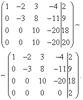
Here is the system of equations.

For convenience, it is better to immediately make her matrix

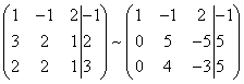
It is known that when solving the Gauss method, the equation corresponding to the first string will remain unchanged at the end of the transformations. Therefore, it will be more profitable if the left upper element of the matrix is \u200b\u200bthe smallest - then the first elements of the remaining lines after operations will turn into zero. So, in the composed matrix, it will be profitable for the first line to put the second line.

second line: k \u003d (-a 21 / a 11) \u003d (-3/1) \u003d -3

a "21 \u003d a 21 + k × a 11 \u003d 3 + (-3) × 1 \u003d 0

a "22 \u003d a 22 + k × a 12 \u003d -1 + (-3) × 2 \u003d -7

a "23 \u003d a 23 + k × a 13 \u003d 1 + (-3) × 4 \u003d -11

b "2 \u003d b 2 + k × b 1 \u003d 12 + (-3) × 12 \u003d -24

third Row: k \u003d (-a 3 1 / a 11) \u003d (-5/1) \u003d -5

a "3 1 \u003d a 3 1 + k × a 11 \u003d 5 + (-5) × 1 \u003d 0

a "3 2 \u003d a 3 2 + k × a 12 \u003d 1 + (-5) × 2 \u003d -9

a "3 3 \u003d A 33 + K × A 13 \u003d 2 + (-5) × 4 \u003d -18

b "3 \u003d b 3 + k × b 1 \u003d 3 + (-5) × 12 \u003d -57

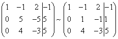
Now, in order not to get confused, you need to record a matrix with intermediate results of transformations.

Obviously, such a matrix can be made more convenient for perception using some operations. For example, from the second line, you can remove all the "minuses", multiplying each element on "-1".

It is also worth noting that in the third line all the elements are multiple three. Then you can reduce the string to this number, multiplying each element to "-1/3" (minus - at the same time to remove negative values).

It looks much more pleasant. Now it is necessary to leave the first string alone and work with the second and third. The task is to add to the third line the second, multiplied by such a coefficient so that the element A 32 becomes zero.

k \u003d (-a 32 / a 22) \u003d (-3/7) \u003d -3/7 (if during some transformations in response it turned out not a whole number, it is recommended to comply with the accuracy of calculations to leave it "as is", in the form of an ordinary Fusi, and only later, when answers received, decide whether it is worth rounding and translate to another form of recording)

a "32 \u003d a 32 + k × a 22 \u003d 3 + (-3/7) × 7 \u003d 3 + (-3) \u003d 0

a "33 \u003d a 33 + k × a 23 \u003d 6 + (-3/7) × 11 \u003d -9/7

b "3 \u003d b 3 + k × b 2 \u003d 19 + (-3/7) × 24 \u003d -61/7

The matrix with new values \u200b\u200bis recorded again.

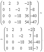
1	2	4	12
0	7	11	24
0	0	-9/7	-61/7

As can be seen, the resulting matrix already has a stepped look. Therefore, further transformations of the Gauss method are not required. What you can do here is to remove the total coefficient "-1/7" from the third line.

Now everything is beautiful. It's small - burn the matrix again in the form of a system of equations and calculate the roots

x + 2y + 4z \u003d 12 (1)

7Y + 11z \u003d 24 (2)

That algorithm for which the roots will be now called back in the Gauss method. In equation (3) contains Z:

y \u003d (24 - 11 × (61/9)) / 7 \u003d -65/9

And the first equation allows you to find X:

x \u003d (12 - 4z - 2y) / 1 \u003d 12 - 4 × (61/9) - 2 × (-65/9) \u003d -6/9 \u003d -2/3

Such a system we have the right to name jointly, and even certain, that is, having a sole decision. The answer is written in the following form:

x 1 \u003d -2/3, y \u003d -65/9, z \u003d 61/9.

An example of an uncertain system

An option for solving a specific system by Gauss method is disassembled, now it is necessary to consider the case if the system is uncertain, that is, you can find infinitely a lot of solutions.

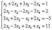
x 1 + x 2 + x 3 + x 4 + x 5 \u003d 7 (1)

3x 1 + 2x 2 + x 3 + x 4 - 3x 5 \u003d -2 (2)

x 2 + 2x 3 + 2x 4 + 6x 5 \u003d 23 (3)

5x 1 + 4x 2 + 3x 3 + 3x 4 - x 5 \u003d 12 (4)

The type of system itself is already alarming, because the number of unknown n \u003d 5, and the rank of the system's matrix is \u200b\u200balready accurately less than this number, because the number of rows M \u003d 4, that is, the largest order of the square-square - 4. So solutions there is an infinite set, and We must look for his general view. The Gauss method for linear equations allows you to do this.

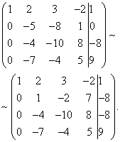
First, as usual, an extended matrix is \u200b\u200bcompiled.

The second line: the coefficient k \u003d (-a 21 / a 11) \u003d -3. In the third line, the first element is before the transformations, so you do not need to touch anything, it is necessary to leave as it is. Fourth line: k \u003d (-a 4 1 / a 11) \u003d -5

Multiplying the elements of the first line for each of their coefficients in turn and folding them with the desired rows, we get a matrix next species:

As you can see, the second, third and fourth lines consist of elements proportional to each other. The second and fourth are generally the same, so one of them can be removed immediately, and the remaining multiply to the coefficient "-1" and get the line number 3. and again from two identical lines to leave one.

It turned out such a matrix. The system has not yet been recorded, it is necessary to determine the basic variables here - standing with coefficients a 11 \u003d 1 and a 22 \u003d 1, and free - all others.

In the second equation there is only one basic variable - x 2. It means that it can be expressed from there by writing through the variables x 3, x 4, x 5, which are free.

We substitute the resulting expression in the first equation.

It turned out the equation in which the only basic variable - x 1. We do the same with it as with x 2.

All basic variables, which are two, are expressed in three free, now you can write the answer in general form.

You can also specify one of the private solutions of the system. For such cases, as a rule, zeros are chosen as values \u200b\u200bfor free variables. Then the answer will be:

16, 23, 0, 0, 0.

An example of an incompatible system

The solution of incomplete systems of equations by Gauss method is the fastest. It ends immediately as soon as one of the steps is obtained equation that has no solution. That is, a stage with the calculation of the roots, a long and vigorous, disappears. The following system is considered:

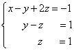
x + Y - Z \u003d 0 (1)

2x - y - z \u003d -2 (2)

4x + y - 3z \u003d 5 (3)

As usual, the matrix is \u200b\u200bcompiled:

1	1	-1	0
2	-1	-1	-2
4	1	-3	5

And drives to the step:

k 1 \u003d -2k 2 \u003d -4

1	1	-1	0
0	-3	1	-2
0	0	0	7

After the first transformation in the third line contains the species equation

not solutions. Consequently, the system is incomplete, and the answer will be empty set.

Advantages and disadvantages of the method

If you choose what method to solve the slam on paper with a handle, then the method that was considered in this article looks most attractive. In elementary transformations, it is much more difficult to get confused than if it happens if you have to search for a manually determinant or some cunning reverse matrix. However, if you use programs for working with data of this type, for example, spreadsheets, it turns out that in such programs the algorithms for calculating the main parameters of matrices are already laid - the determinant, minors, reverse and so on. And if you confident that the car counts these values \u200b\u200bitself and will not be mistaken, it is advisable to use the matrix method or the crawler formula, because their use begins and ends with the calculation of determinants and inverse matrices.

Application

Since the solution by the Gauss method is an algorithm, and the matrix is, in fact, a two-dimensional array, it can be used when programming. But since the article positions itself as a guide "for teapots", it should be said that the simplest thing is where the method can be stuffed - these are spreadsheets, for example, Excel. Again, all sorts of slows listed in the table in the form of a matrix, Excel will be considered as a two-dimensional array. And for operations with them there are many pleasant teams: addition (you can only fold the matrices of the same sizes!), Multiplication by the number, multiplying matrices (also with certain limitations), finding back and transposed matrices and, most importantly, calculating the determinant. If this time-consuming occupation is replaced by one team, it is possible to determine the rag of the matrix much faster and, therefore, to establish its unity or incompleteness.

Gauss method Perfect for solving systems of linear algebraic equations (Slava). It has a number of advantages over other methods:

• first, there is no need to pre-explore the system of equations for units;
• secondly, the Gauss method can be solved not only to the slope in which the number of equations coincides with the number of unknown variables and the main matrix of the system is non-degenerate, but also the system of equations in which the number of equations does not coincide with the number of unknown variables or the determinant of the main matrix is \u200b\u200bzero;
• thirdly, the Gauss method leads to a result with a relatively small number of computing operations.

A brief overview of the article.

First, we will give the necessary definitions and introduce notation.

Next, we describe the algorithm of the Gauss method for the simplest case, that is, for systems of linear algebraic equations, the number of equations in which coincides with the number of unknown variables and the determinant of the main matrix of the system is not zero. When solving such systems of equations, the essence of the Gauss method is most clearly visible, which is consistent with the exclusion of unknown variables. Therefore, Gauss method is also called the method of consistent exclusion of unknown. Show detailed solutions several examples.

In conclusion, we consider the solution by the Gauss method of linear algebraic equations, the main matrix of which is either rectangular or degenerate. The solution of such systems has some features that we will analyze in detail on the examples.

Navigating page.

Basic definitions and designations.

Consider the system from p linear equations with n unknown (P may be equal to N):

Where - unknown variables - numbers (valid or complex), - free members.

If a then the system of linear algebraic equations is called uniform, otherwise - heterogeneous.

The combination of the values \u200b\u200bof unknown variables in which all system equations are treated in identities, is called decision of the slown.

If there is at least one solution of a system of linear algebraic equations, then it is called joint, otherwise - non-stop.

If the Slava has a single decision, then it is called defined. If the solutions are more than one, then the system is called uncertain.

It is said that the system is recorded in coordinate formif it has the view
.

This system B. matrix form records has a view where - the main matrix of the Slava, - the matrix column of unknown variables, is the matrix of free members.

If you add to the matrix and add a matrix-column-column of free members, then we get the so-called extended matrix Systems of linear equations. Typically, the expanded matrix is \u200b\u200bdenoted by the letter T, and the column of free members is separated by the vertical line from the remaining columns, that is,

Square matrix A called degenerateif its determinant is zero. If, then the matrix is \u200b\u200bcalled non-degenerate.

The next moment should be stated.

If the system of linear algebraic equations make the following actions

• swap two equations
• multiply both parts of any equation on an arbitrary and non-zero valid (or complex) number k,
• to both parts of any equation to add the corresponding parts of another equation multiplied by an arbitrary number k,

it will turn out an equivalent system that has the same solutions (or also as the source does not have solutions).

For an extended matrix of a system of linear algebraic equations, these actions will mean conducting elementary transformations with lines:

• rearrange two lines in places
• multiplying all elements of any row of the matrix T to different from zero number k,
• add to elements of any row of the matrix of the corresponding elements of another line multiplied by an arbitrary number k.

Now you can go to the description of the Gauss method.

Solving systems of linear algebraic equations in which the number of equations is equal to the number of unknown and the main matrix of the system is non-degenerate, by Gauss method.

How would we enroll in school if you got the task to find the solution of the system of equations .

Some would have done so.

Note that adding the left part of the first to the left side of the second equation, and the right part is right, you can get rid of unknown variables x 2 and x 3 and immediately find X 1:

We substitute the found value x 1 \u003d 1 in the first and third system equation:

If you multiply both parts of the third system equation on -1 and add them to the corresponding parts of the first equation, then we will get rid of an unknown variable x 3 and be able to find X 2:

We substitute the obtained value x 2 \u003d 2 in the third equation and find the remaining unknown variable x 3:

Others would have accepted otherwise.

Allowing the first system equation relative to an unknown variable x 1 and substitute the resulting expression in the second and third system equation to eliminate this variable from them:

Now allowing the second system equation relative to X 2 and substitute the result obtained in the third equation to exclude an unknown variable x 2 from it:

From the third equation of the system it can be seen that x 3 \u003d 3. Find from the second equation , and from the first equation we get.

Familiar solutions, isn't it?

The most interesting thing is that the second way to solve is essentially a method of consistent exclusion of unknown, that is, the Gauss method. When we expressed unknown variables (first x 1, in the next step x 2) and substituted them into the remaining equations of the system, we thus excluded them. The exception we carried out until one unknown variable remained in the last equation. The process of consistent exclusion of unknowns is called direct running of the Gauss method. After completing the direct course, we appear the ability to calculate an unknown variable in the last equation. With its help, from the penultimate equation, we find the next unknown variable and so on. The process of consistent finding unknown variables when moving from the last equation to the first one is called return of the Gauss method.

It should be noted that when we express X 1 through x 2 and x 3 in the first equation, and then we substitute the obtained expression into the second and third equations, then the following actions lead to the same result:

Indeed, such a procedure also eliminates the unknown variable x 1 from the second and third system equations:

The nuances with the exception of unknown variables by the Gauss method occur when the system equations do not contain some variables.

For example, in a slope In the first equation there is no unknown variable x 1 (in other words, the coefficient in front of it is zero). Therefore, we cannot solve the first system equation relative to X 1 to eliminate this unknown variable from the remaining equations. The exit from this situation is the permutation of the system equations. Since we consider the system of linear equations, the determinants of the main matrices of which are different from zero, there is always an equation in which the variable you need is present, and we can rearrange this equation to the position we need. For our example, it is enough to change the first and second system equations. Moreover, you can resolve the first equation relative to X 1 and exclude it from the remaining system equations (although there is no already absent in the second equation).

We hope that the essence you caught.

We describe algorithm of Gauss method.

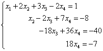
Let us need to solve the system from n linear algebraic equations with n unknown variables , And let the determinant of its main matrix differ from zero.

We will assume that, since we can always achieve this permutation of the system equations. Except an unknown variable x 1 of all equations of the system, starting from the second. To do this, the second equation of the system will add the first, multiplied by, to the third equation, add the first, multiplied by, and so on, to the N-th equation to add the first, multiplied by. The system of equations after such transformations will take the form

where, A. .

We would have come to the same result if X 1 would expressed X 1 through other unknown variables in the first equation of the system and the resulting expression substituted into all other equations. Thus, the variable x 1 is excluded from all equations, starting from the second.

Next, we act likewise, but only with a part of the obtained system, which is marked in the figure

To do this, we add the second, multiplied by, to the fourth equation to the fourth equation, the second, multiplied by, and so on, to the N-th equation, add the second, multiplied by. The system of equations after such transformations will take the form

where, A. . Thus, the variable x 2 is excluded from all equations, starting from the third.

Next, proceed to the exclusion of an unknown X 3, while acting similarly to the part of the system marked in the figure

So we continue the direct move of the Gauss method while the system does not take

From that moment, we begin the reverse course of the Gauss method: Calculate the X N from the last equation, as using the resulting X N, we find X N-1 from the penultimate equation, and so on, we find x 1 from the first equation.

We will analyze the algorithm on the example.

Example.

Gauss method.

Decision.

The A 11 coefficient is different from zero, so we will proceed to the direct move of the Gauss method, that is, to the exclusion of an unknown variable x 1 of all equations of the system, except for the first. To do this, to the left and right parts of the second, third and fourth equation, add the left and right parts of the first equation multiplied by respectively and:

The unknown variable x 1 was excluded, go to the exception of X 2. To the left and right parts of the third and fourth equations of the system add the left and right parts of the second equation, multiplied by respectively and :

To complete the direct movement of the Gauss method, we have left to exclude an unknown variable x 3 from the last equation of the system. Add to the left and right parts of the fourth equation, respectively, the left and right side of the third equation multiplied by :

You can begin the opposite course of the Gauss method.

From the last equation we have ,
From the third equation we get
from the second
From the first.

To check, you can substitute the obtained values \u200b\u200bof unknown variables to the source system of equations. All equations are treated in identities, which indicates that the decision on the Gauss method is found true.

Answer:

And now we present the solution of the same example by the Gauss method in the matrix form of recording.

Example.

Find a solution to the system of equations Gauss method.

Decision.

Extended system matrix has the view . From above over each column, unknown variables are recorded, which correspond to the elements of the matrix.

The direct stroke of the Gauss method here implies the enhanced system matrix to the trapezoidal type using elementary transformations. This process is similar to the exception of unknown variables that we conducted with the system in coordinate form. Now you will make sure that.

We transform the matrix so that all the elements in the first column starting from the second are zero. To do this, to elements of the second, third and fourth lines add the corresponding elements of the first line multiplied by, And on respectively:

Further, the resulting matrix is \u200b\u200bconverting so that in the second column all the elements, starting from the third steel zero. This will correspond to the exclusion of an unknown variable x 2. To do this, add the corresponding elements of the first line of the matrix to the elements of the third and fourth lines, multiplied by respectively and :

It remains to exclude an unknown variable x 3 from the last system equation. To do this, to elements of the last line of the resulting matrix add the appropriate elements of the penultimate line multiplied by :

It should be noted that this matrix corresponds to the system of linear equations.

Which was obtained earlier after direct stroke.

The reverse time has come. In the matrix form of recording, the reverse move of the Gauss method involves such a conversion of the resulting matrix to the matrix marked in the figure

became diagonal, that is, took the view

Where are some numbers.

These transformations are similar to the transformations of the direct movement of the Gauss method, but are not performed from the first string to the latter, but from the last to the first.

I add to the elements of the third, second and first lines the corresponding elements of the last line multiplied by , on and on respectively:

Now add to the elements of the second and first lines the corresponding elements of the third line multiplied by and on respectively:

At the last step of the reverse movement of the Gauss method to the elements of the first line add the corresponding elements of the second line multiplied by:

The resulting matrix corresponds to the system of equations Where we find unknown variables.

Answer:

NOTE.

When using the Gauss method to solve linear algebraic equations, approximate calculations should be avoided, as this can lead to absolutely incorrect results. We recommend not rounding decimal fractions. Better from decimal fractions to move to ordinary fractions.

Example.

Solve a system of three equations by Gauss .

Decision.

Note that in this example, unknown variables have a different designation (not x 1, x 2, x 3, and x, y, z). Let us turn to ordinary fractions:

Except unknown X from the second and third equations of the system:

In the resulting system in the second equation there is no unknown variable y, and in the third equation Y is present, therefore, rearrange the second and third equations in some places:

On this, the direct stroke of the Gauss method is over (from the third equation it is not necessary to exclude Y, since this unknown variable is no longer).

Get on the opposite move.

I find from the last equation ,
From the penultimate


From the first equation we have

Answer:

X \u003d 10, y \u003d 5, z \u003d -20.

Solving systems of linear algebraic equations in which the number of equations does not coincide with the number of unknown or the main matrix of the system degenerate, the Gauss method.

Systems of equations, the main matrix of which is rectangular or square degenerate, may not have solutions, may have a single solution, and may have infinite set solutions.

Now we will understand how the Gauss method allows you to establish allocate or incompleteness of the system of linear equations, and in the case of its compatibility, it is necessary to determine all solutions (or one single solution).

In principle, the process of excluding unknown variables in the case of such a slope remains the same. However, it is necessary to stay in detail on some situations that may arise.

Go to the most important stage.

So, we assume that the system of linear algebraic equations after the completion of the direct movement of the Gauss method took And no equation was reduced to (in this case, we would conclude about system incompleteness). There is a logical question: "What to do next"?

We discard unknown variables that are in the first place of all equations of the obtained system:

In our example, it is x 1, x 4 and x 5. In the left parts of the system equations, we only leave those components that contain the discharged unknown variables x 1, x 4 and x 5, the rest of the components are transferred to the right side of the equations with the opposite sign:

Give unknown variables that are in the right parts of equations, arbitrary values \u200b\u200bwhere - Arbitrary numbers:

After that, in the right parts of all the equations of our Slava, there are numbers and it is possible to crime to the opposite move of the Gauss method.

From the last equations of the system, we have, from the penultimate equation we find, from the first equation we get

By solving the system of equations, the set of unknown variables values

Giving numbers Various values, we will receive various solutions of the equation system. That is, our system of equations has infinitely many solutions.

Answer:

Where - Arbitrary numbers.

To secure the material in detail the solutions of several more examples.

Example.

Solve a homogeneous system of linear algebraic equations Gauss method.

Decision.

Except an unknown variable x from the second and third system equations. To do this, to the left and right part of the second equation, according to the left and right parts of the first equation, multiplied by, and to the left and right side of the third equation, the left and right parts of the first equation are multiplied by:

Now we will exclude Y from the third equation of the system of equations:

The resulting Slava is equivalent to the system .

We leave on the left part of the system equations only the terms containing unknown variables X and Y, and the terms with an unknown variable z are transferred to the right side:

The Gauss method, also called the method of consistent exclusion of unknown, is as follows. With the help of elementary transformations, the system of linear equations lead to this species so that its matrix from the coefficients is trapezoidal (the same as triangular or stepped) or close to the trapezoidal (the direct move of the Gauss method, then it's just a direct move). An example of such a system and its solution - in the picture from above.

In such a system, the latter equation contains only one variable and its value can be unambiguously found. Then the value of this variable is substituted into the previous equation ( return of the Gauss method Further - just the reverse), from which the previous variable finds, and so on.

In the trapezoidal (triangular) system, as we see, the third equation no longer contains variables y. and x. , and the second equation - variable x. .

After the system's matrix took a trapezoidal form, it is no longer possible to understand the issue of the system's compatibility, to determine the number of solutions and find the decisions themselves.

Benefits of the method:

1. when solving systems of linear equations with the number of equations and unknown more than three, the Gauss method is not as cumbersome as the Cramer method, since when solving the Gauss method, less computations are necessary;
2. the Gauss method can solve indefinite systems of linear equations, that is, having a general solution (and we will analyze them in this lesson), and using the craver method, you can only state that the system is uncertain;
3. systems of linear equations can be solved, in which the number of unknown persons is not equal to the number of equations (we will also analyze them in this lesson);
4. the method is based on elementary (school) methods - the method of substitution of unknown and the method of addition of the equations that we touched in the relevant article.

So that everyone is imbued with simplicity, with which trapezoidal (triangular, speed) systems of linear equations are solved, we will give the solution to such a system using reverse stroke. The rapid solution of this system was shown in the picture at the beginning of the lesson.

Example 1. Solve the system of linear equations, applying the reverse move:

Decision. In this trapezoidal system variable z. Definitely located from the third equation. We substitute its value into the second equation and get the value of the variable y.:

Now we know the values \u200b\u200bof two variables - z. and y.. We substitute them in the first equation and get the value of the variable x.:

From previous steps, we write out the solution of the system of equations:

In order to obtain such a trapezoidal system of linear equations, which we decided very simply, it is necessary to apply a direct course associated with elementary transformations of a system of linear equations. It is also not very difficult.

Elementary transformations of a system of linear equations

Repeating the school method of algebraic addition equations of the system, we found out that one system of the system can be added to one of the equations of the system, and each of the equations can be multiplied by some numbers. As a result, we obtain a system of linear equations equivalent to this. It already contained only one variable, substituting the value of which to other equations, we arrive at the solution. Such addition is one of the types of elementary system conversion. When using the Gauss method, we can use several types of transformations.

On the animation above, it is shown as the system of equations gradually turns into a trapezoidal one. That is, that you have seen on the very first animation and were convinced that it was just to find the values \u200b\u200bof all unknown. About how to perform such a transformation and, of course, examples will be discussed.

When solving systems of linear equations with any number of equations and unknown in the system of equations and in the extended matrix of the system can:

1. rearrange the line in places (this was mentioned at the very beginning of this article);
2. if, as a result of other transformations, equal or proportional lines appeared, they can be removed, except one;
3. remove the "zero" lines, where all the coefficients are zero;
4. any string multiply or divide for a number;
5. to any row, add another string multiplied by a number.

As a result of the transformations, we obtain a system of linear equations equivalent to this.

Algorithm and examples of solving Gauss method of linear equations with a square matrix system

Consider first the solution of systems of linear equations, in which the number of unknown is equal to the number of equations. The matrix of such a system is square, that is, in it the number of rows is equal to the number of columns.

Example 2. Solve Gauss method of linear equations

Solving systems of linear equations school methods, we have multiplied one of the equations for a certain number so that the coefficients at the first variable in the two equations were opposite. When the equations are addition, this variable is eliminated. The Gauss method is also valid.

For simplification external view solutions make an extended system matrix:

In this matrix to the left to the vertical feature there are coefficients at unknown, and on the right after the vertical feature - free members.

For the convenience of dividing coefficients with variables (to obtain division per unit) rearrange the first and second lines of the system matrix. We obtain the system equivalent to this, since the system of linear equations can be rearranged by places of the equation:

With the help of a new first equation let us excel the variable x. from the second and all subsequent equations. To do this, the second line of the matrix add the first line multiplied by (in our case), to the third line - the first line multiplied by (in our case).

It is possible because

If there were more than three equations in our system of equations, it would be necessary to add to all subsequent equations to the first line multiplied by the ratio of the respective coefficients taken with a minus sign.

As a result, we obtain the matrix equivalent to this system of the new system of equations in which all equations starting from the second do not contain variables x. :

To simplify the second row of the obtained system, I multiply it on and we obtain the matrix of the system of equations equivalent to this system:

Now, while maintaining the first equation of the obtained system without changes, using the second equation, we exclude a variable y. Of all subsequent equations. To do this, we add a second string multiplied by the system to the third line of the system, multiplied by (in our case).

If there were more than three equations in our system of equations, it would be necessary to add to all subsequent equations to the second line multiplied by the ratio of the respective coefficients taken with a minus sign.

As a result, we again obtain the system matrix equivalent to this system of linear equations:

We received an equivalent to this trapezoidal system of linear equations:

If the number of equations and variables are greater than in our example, the process of consistent exception of variables continues until the system matrix becomes a trapezoidal, as in our demo example.

Decision will find "from the end" - reverse. For this from the last equation we define z.:
.
Substituting this value into the preceding equation, find y.:

From the first equation find x.:

Answer: Solution of this system of equations - .

: In this case, the same answer will be issued if the system has a definite solution. If the system has an infinite set of solutions, then there will be a response, and this is the subject of the fifth of this lesson.

Solve the system of linear equations by the Gauss method independently, and then see the decision

We are once again an example of a joint and defined system of linear equations, in which the number of equations is equal to the number of unknown. The difference from our demo-example from the algorithm is already four equations and four unknown.

Example 4. Solve the system of linear equations by Gauss:

Now you need to eliminate the variable from the subsequent equations using the second equation. Cut preparatory work. To be more convenient with the attitude of the coefficients, you need to get a unit in the second column of the second string. To do this, from the second line will be read the third, and as a result, the second line multiply by -1.

We now actually eliminate the variable from the third and fourth equations. To do this, add the second line to the third line, multiplied by, and the fourth - the second, multiplied by.

Now with the help of the third equation, we will exclude a variable from the fourth equation. To do this, add the third, multiplied by the fourth line. We get an extended trapezoidal form matrix.

Received a system of equations that the specified system is equivalent:

Consequently, the obtained and this system are joint and defined. Final solution to find "From the end". From the fourth equation, we can directly express the value of the variable "X fourth" variable:

This value is substituted in the third equation of the system and get

,

,

Finally, substitution of values

In the first equation gives

,

where we find "Iks first":

Answer: This system of equations has the only solution. .

Check the system solution can also be on the Calculator decisive by the Cramer: In this case, the same answer will be issued if the system has an unambiguous solution.

Solving the Gauss method of applied tasks on the example of the task on the alloys

Systems of linear equations are used to simulate real objects of the physical world. We decide one of these tasks - on alloys. Similar tasks - tasks for mixtures, cost or specific gravity individual goods in the group of goods and the like.

Example 5.Three pieces of alloy have a total weight of 150 kg. The first alloy contains 60% of copper, the second is 30%, the third is 10%. At the same time, in the second and third alloys together, copper taken by 28.4 kg less than in the first alloy, and in the third copper alloy by 6.2 kg less than in the second. Find a lot of every piece of alloy.

Decision. We compile a system of linear equations:

We multiply the second and third equations by 10, we obtain an equivalent system of linear equations:

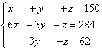
We compile an extended system matrix:

Attention, direct move. By addition (in our case, subtraction) of one line multiplied by the number (apply two times) with an extended matrix of the system, the following transformations occur:

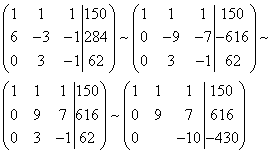
The direct move ended. Received an extended matrix of trapezoidal form.

Apply the reverse move. We find a solution from the end. We see that.

Find from the second equation

From the third equation -

You can check the system solution on the Calculator decisive by the Cramer method: in this case, the same answer will be issued if the system has a unambiguous solution.

The simplicity of the Gauss method speaks at least the fact that the German mathematics Karl Friedrich Gaussu requires only 15 minutes to his invention. In addition to the method of his name from Creativity Gauss, the saying is known "should not be mixed what it seems to us incredible and unnatural, with absolutely impossible" - a kind brief instructions For the performance of discoveries.

In many applied tasks, it may not be a third limitation, that is, the third equation, then it is necessary to solve the Gauss method of two equations with three unknown, or, on the contrary, unknown less than equations. We now proceed to solve such systems of equations.

With the help of the Gauss method, you can install, shared or inconsistent any system n. Linear Equations S. n. variables.

Gauss method and system of linear equations having infinite set solutions

The following example is a joint, but indefinite system of linear equations, that is, having infinite set solutions.

After performing the transformations in an extended system matrix (permutations of strings, multiplication and dividing strings for a number, adding to one line, the rows of the form could appear

If in all equations of

Free members are zero, this means that the system is undefined, that is, it has an infinite set of solutions, and the equations of this species are "extra" and exclude them from the system.

Example 6.

Decision. Make an extended system matrix. Then, with the help of the first equation, we exclude a variable from subsequent equations. To do this, to the second, third and fourth rows add the first, multiplied according to:

Now I will add a second line to the third and fourth.

As a result, we arrive at the system

The last two equations turned into the view equations. These equations are satisfied with any values \u200b\u200bof unknown and they can be discarded.

To satisfy the second equation, we can for and choose arbitrary values, then the value for it is already definitely determined: . From the first equation, the value for also is definitely: .

Both the given and last systems are jointly, but uncertain, and formulas

for arbitrary and give us all solutions of a given system.

Gauss method and system of linear equations that do not have solutions

The following example is an incomplete system of linear equations, that is, non-solutions. The answer to such tasks is formulated: the system has no solutions.

As mentioned in connection with the first example, after performing transformations in an extended matrix of the system, the strings of the form could appear

corresponding equation of species

If there are at least one equation with a free member different from zero (i.e.), then this system of equations is incomplete, that is, it does not have solutions and its decision is completed.

Example 7. Solve the Gauss method of linear equations:

Decision. We compile an extended system matrix. Using the first equation, we exclude from subsequent variable equations. To do this, the second line add the first, multiplied by, to the third line - the first, multiplied by, to the fourth - the first, multiplied by.

Now you need to eliminate the variable from the subsequent equations using the second equation. To obtain entire ratio of coefficients, change the second and third lines of the extended system matrix in places.

To exclude from the third and fourth equation to the third line add the second, multiplied by, and to the fourth - the second, multiplied by.

Now with the help of the third equation, we will exclude a variable from the fourth equation. To do this, add the third, multiplied by the fourth line.

The specified system is equivalent, thus as follows:

The resulting system is incomplete, since its last equation cannot be satisfied with any values \u200b\u200bof unknown. Consequently, this system has no solutions.

Let a system of linear algebraic equations, which must be solved (to find such values \u200b\u200bof unknown XI, resulting in each system equation into equality).

We know that the system of linear algebraic equations can:

1) not to have solutions (be non-stop).
2) have infinitely many solutions.
3) to have a single solution.

As we remember, the cramer rule and the matrix method are produced in cases where the system has infinitely a lot of solutions or incomplete. Gauss method – the most powerful and universal tool for finding a solution of any system of linear equations, which the in each casewill lead us to the answer! The algorithm of the method itself in all three cases works equally. If knowledge of determinants are needed in the Cramer methods and the matrix, then the knowledge of only arithmetic action is needed to use the Gauss method, which makes it affordable even for primary school students.

Converting an extended matrix ( this is the system matrix - a matrix, compiled only from coefficients at unknown, plus a column of free members)linear algebraic equations in the Gauss method:

1) from troch Matrians can rearrangeplaces.

2) if the matrix appeared (or there) proportional (as a special case - the same) lines, then delete From the matrix all these lines besides one.

3) If a zero string appeared in the matrix during the conversion, it should also delete.

4) the matrix string can be multiply (divided)for any number other than zero.

5) to the string of the matrix add another string multiplied by the numberdifferent from zero.

In the Gauss method, elementary transformations do not change the solution of the system of equations.

The Gauss method consists of two stages:

1. "Direct stroke" - with the help of elementary transformations, lead an extended matrix of a system of linear algebraic equations to the "triangular" step: elements of the extended matrix, located below the main diagonal, are zero (the move "top-down"). For example, to this species:

To do this, do the following:

1) Let we consider the first equation of a system of linear algebraic equations and the coefficient at x 1 is K. second, third, etc. Equations are converting as follows: Each equation (coefficients at unknown, including free terms) divide on the coefficient at an unknown X 1, which is in each equation, and multiply on K. After that, from the second equation (coefficients with unknown and free members), we subtract first. We obtain at x 1 in the second equation, the coefficient of 0. From the third transformed equation, we submit the first equation, so as long as all equations except the first, with an unknown X 1, will not have a coefficient of 0.

2) Go to the next equation. Let it be the second equation and the coefficient at X 2 is M. with all the "lower-level" equations in the same way as described above. Thus, "under" unknown X 2 in all equations will zero.

3) Go to the next equation and so before it is time until one last unknown and transformed free member remain.

1. "Return" method of Gauss - obtaining a solution of a system of linear algebraic equations ("bottom-up" stroke). From the last "lower" equation, we obtain one first solution - an unknown x n. To do this, we solve the elementary equation A * x n \u003d V. In the example above, x 3 \u003d 4. We substitute the value found in the "upper" the following equation and solve it relative to the next unknown. For example, x 2 - 4 \u003d 1, i.e. x 2 \u003d 5. And so until we find all unknown.

Example.

We decide the system of linear equations by Gauss method, as some authors advise:

We write the expanded matrix of the system and with the help of elementary transformations we give it to the step type:

We look at the left upper "step". There we must have a unit. The problem is that there are no units in the first column at all, so nothing to solve the permutation of the rows. In such cases, one needs to be organized using an elementary transformation. This can usually be done in several ways. Let's do this:
1 step . To the first line add the second string multiplied by -1. That is, mentally multiplied the second line on -1 and completed the addition of the first and second line, while we did not change the second line.

Now on the left at the top of "minus one" that it is quite suitable. Who wants to get +1, can perform an additional action: multiply the first string on -1 (change the sign from it).

2 step . To the second line added the first line multiplied by 5. To the third line added the first string multiplied by 3.

3 Step . The first line was multiplied by -1, in principle, it is for beauty. The third line also changed the sign and rearranged it in second place, so on the second "step we had the desired unit.

4 Step . The third line added a second string multiplied by 2.

5 step . The third line was divided into 3.

The feature that indicates an error in calculations (less often about typing) is the "bad" bottom line. That is, if we had something like something like (0 0 11 | 23), and, respectively, 11x 3 \u003d 23, x 3 \u003d 23/11, then with a large share of probability it can be argued that an error is allowed during Elementary transformations.

We carry out the opposite move, in the design of examples often do not rewrite the system itself, and the equations "take directly from the above matrix". Return, I remind, works "bottom up". In this example, a gift turned out:

x 3 \u003d 1
x 2 \u003d 3
x 1 + x 2 - x 3 \u003d 1, therefore x 1 + 3 - 1 \u003d 1, x 1 \u003d -1

Answer: x 1 \u003d -1, x 2 \u003d 3, x 3 \u003d 1.

Let the same system on the proposed algorithm. Receive

4 2 –1 1
5 3 –2 2
3 2 –3 0

We divide the second equation on 5, and the third - by 3. We get:

4 2 –1 1
1 0.6 –0.4 0.4
1 0.66 –1 0

Multiply the second and third equations for 4, we get:

4 2 –1 1
4 2,4 –1.6 1.6
4 2.64 –4 0

Subscribe from the second and third equations the first equation, we have:

4 2 –1 1
0 0.4 –0.6 0.6
0 0.64 –3 –1

We divide the third equation by 0.64:

4 2 –1 1
0 0.4 –0.6 0.6
0 1 –4.6875 –1.5625

Multiply the third equation by 0.4

4 2 –1 1
0 0.4 –0.6 0.6
0 0.4 –1.875 –0.625

The second equation will be subtracted from the third equation, we get a "stepped" expanded matrix:

4 2 –1 1
0 0.4 –0.6 0.6
0 0 –1.275 –1.225

Thus, since the error was accumulated in the calculation process, we obtain x 3 \u003d 0.96 or approximately 1.

x 2 \u003d 3 and x 1 \u003d -1.

Slimming in this way, you never confuse in the calculations and despite the calculation errors, get the result.

This method of solving a system of linear algebraic equations is easily programmed and does not take into account the specific features of the coefficients at unknown, because in practice (in economic and technical calculations), it is necessary to deal with the neuroble coefficients.

I wish you success! See you in class! Tutor Dmitry Iistakhanov.

the site, with full or partial copying of the material reference to the original source is required.

One of the simplest ways to solve the linear equation system is a reception based on the calculation of determinants ( kramer rule). Its advantage is that it allows you to immediately record the solution, especially it is convenient in cases where the system coefficients are not numbers, but by some parameters. Its disadvantage is the bulkness of calculations in the case of a large number of equations, besides, the craver rule is not directly applicable to systems that the number of equations does not coincide with the number of unknown. In such cases, usually apply gauss method.

System of linear equations having the same set of solutions called equivalent. Obviously, the set of solutions of the linear system will not change if any equations change places, or multiply one of the equations for any non-zero number, or if one equation is added to another.

Gauss method (the method of consistent exclusion of unknown) It is that with the help of elementary transformations, the system is driven to an equivalent system of stepped species. First, using the 1st equation is excluded x. 1 of all subsequent system equations. Then with the help of the 2nd equation is excluded x. 2 of the 3rd and all subsequent equations. This process, called direct running of the Gauss method, continues until only one unknown in the left part of the last equation remains x N.. After that produced return of the Gauss method - solving the last equation, we find x N.; After that, using this value, from the penultimate equation, calculate x N. -1, etc. The latter are found x. 1 of the first equation.

Gauss transformations are conveniently carried out by conversion not with the equations themselves, but with matrices of their coefficients. Consider the matrix:

called extended system matrix, For in it, except for the main matrix of the system, the column of free members is included. The Gauss method is based on bringing the main matrix of the system to a triangular form (or a trapezoidal form in the case of non-square systems) with the help of elementary string transforms (!) Extended system matrix.

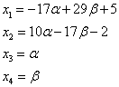
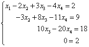
Example 5.1. Solve the system by Gauss:

Decision. We repel the expanded system matrix and, using the first string, after that we will reset the remaining items:

we get zeros in the 2nd, 3rd and 4th lines of the first column:

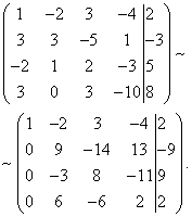
Now it is necessary that all elements in the second column below the 2nd row are zero. To do this, you can multiply the second string to -4/7 and add to the 3rd line. However, in order not to deal with the fractions, create a unit in the 2nd line of the second column and only

Now, to get a triangular matrix, you need to reset the element of the fourth line of the 3rd column, for this you can multiply the third line by 8/54 and add it to the fourth. However, in order not to deal with the fractions, we will change the 3rd and 4th rows and the 3rd column in places and the 4th column and only after that it will be resetting the specified item. Note that when the columns are permutable, the corresponding variables change and need to remember this; Other elementary transformations with columns (addition and multiplication by number) can be produced!

The last simplified matrix corresponds to the equation system equivalent to the initial:

From here, using the reverse move of the Gauss method, we will find from the fourth equation x. 3 \u003d -1; From the third x. 4 \u003d -2, from the second x. 2 \u003d 2 and from the first equation x. 1 \u003d 1. In the matrix form, the answer is written as

We considered the case when the system is defined, i.e. When there is only one solution. Let's see what happens if the system is incomprehensible or uncertain.

Example 5.2. Explore the system by Gauss:

Decision. We write out and transform an extended system matrix

We write down the simplified system of equations:

Here, in the last equation it turned out that 0 \u003d 4, i.e. contradiction. Consequently, the system has no solution, i.e. she is uncomfortable. à

Example 5.3. Explore and solve the system by Gauss:

Decision. We write out and transform an extended system matrix:

As a result of transformations, some zeros turned out in the last row. This means that the number of equations has decreased by one:

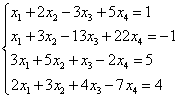
Thus, after simplifications, two equations remained, and unknown four, i.e. Two unknown "unnecessary". Let "superfluous", or, as they say, free variables, be x. 3 I. x. four . Then

Believed x. 3 = 2a. and x. 4 = b., get x. 2 = 1–a. and x. 1 = 2b.–a.; or in matrix form

The decision recorded in this way is called commonbecause, giving parameters a. and b. Various values, you can describe all possible system solutions. à.